What is a Decision Tree?
Decision Trees help you choose between multiple outcomes/courses you might take in a business scenario. They are very visual and help the user understand the risks and rewards associated with each choice (1).
Elements of a Decision Tree
The diagram on the left shows the most basic elements that make up a decision tree:
First, the square nodes represent decisions to be made. These are the decisions that you can make with certainty. The square labeled with 1 here is a decision. The branches coming out of square 1 lead to the different options that you have as a result of making decision 1. Circles A and B are these options, and the circles around them represent uncertainty as to what outcomes might happen. Unlike the squares, which have certainty, these circles represent external events that you have no control over. Each path you take, from left to right, leads to a different outcome. In this case, there are 7 different outcomes with expected values calculated by the user to help understand the process. Once your decision tree is completely made and drawn out, quantitative numbers associated with those outcomes can help you decide which decision is best for you (2).
Let’s go into more depth concerning the layout of decision trees:
A Simple Decision Tree Problem
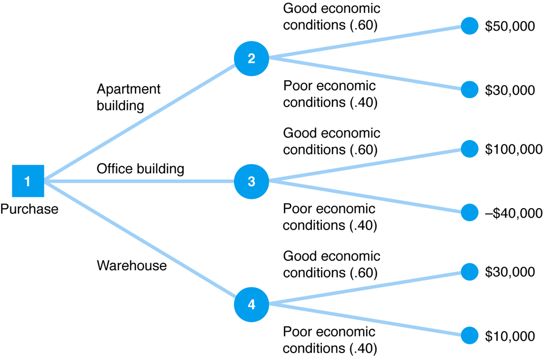
This decision tree illustrates the decision to purchase either an apartment building, office building, or warehouse. Since this is the decision being made, it is represented with a square and the branches coming off of that decision represent 3 different choices to be made. Circles 2, 3, and 4 represent probabilities in which there is uncertainty involved. The branches coming off of the circles show 2 states of nature that are possible: good economic conditions and poor economic conditions. It states here that there is a 60% chance that there will be good economic conditions and a 40% chance that there will be poor economic conditions. To further explain, at node 2, the payoff for a 60% chance of good economic conditions is $50,000. These probabilities may not be known with absolute certainty, so the decision maker might have to estimate the probability of these conditions arising. To determine whether to purchase the apartment building, office building, or warehouse, the decision maker must compute the expected value at each probability (or circle) node.
To compute the expected value at each node, the decision maker will work backward:
Expected value = (Probability of good economic conditions * Payoff associated with that probability) + (Probability of poor economic conditions * Payoff associated with that probability)
Expected value (at node 2): 0.60($50,000) + 0.40($30,000) = $42,000
Expected value (at node 3): 0.60($100,000) + 0.40(-$40,000) = $44,000
Expected value (at node 4): 0.60($30,000) + 0.40($10,000) = $22,000
These expected values are then written over top their corresponding nodes in a square box for easy-access and understanding:
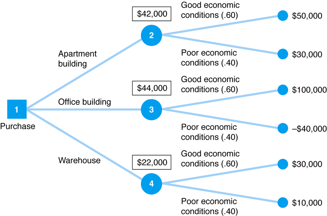
The purchase we choose is whichever node has the expected value that results in the highest payoff. In this case, it is node 3, with an expected payoff of $44,000 (3).
This is a very simple problem, so let’s try a harder one to help better explain decision trees:
This is a very simple problem, so let’s try a harder one to help better explain decision trees:
A More Complicated Problem
Problem:
You go to the racetrack and are choosing between 2 horses: Belle and Jeb. Someone comes and offers you gambler’s anti-insurance. If you agree to it,
· They pay you $2 up front
· You agree to pay them 50% of any winnings (that is, $0.50 if Belle wins, and $5 if Jeb wins).
You can:
· Bet on Belle. It costs $1 to place a bet; you will be paid $2 if she wins (or a net profit of $1).
· Bed on Jeb. It costs $1 to place a bet; you will be paid $11 if he wins (for a net profit of $10).
You believe that Belle has a probability 0.7 of winning and that Jeb has a probability 0.1 of winning.
Solution:
Explanation:
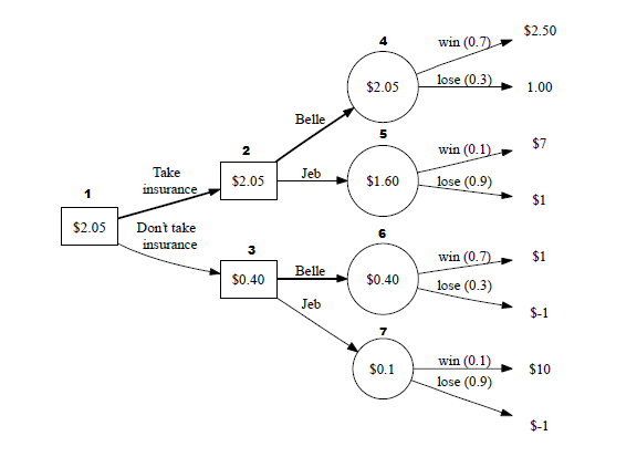
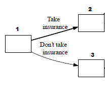
Starting at decision node 1, there are two decisions to be made that are known with certainty: should we take the insurance or not take the insurance? The decision node squares 2 and 3 are where we will put the profit we will make associated with each of the choices.
Starting at decision node 1, there are two decisions to be made that are known with certainty: should we take the insurance or not take the insurance? The decision node squares 2 and 3 are where we will put the profit we will make associated with each of the choices.
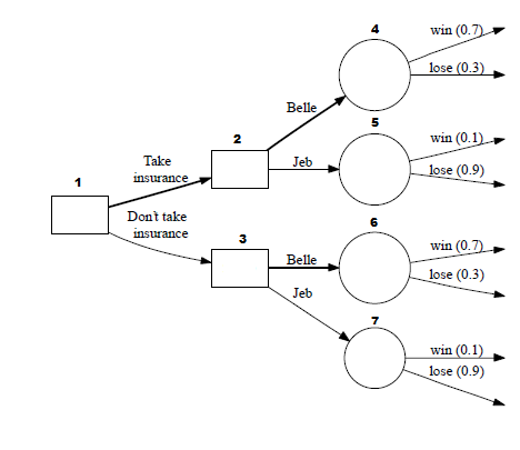
Then branching off of that, there are two choices at each decision square: do we bet on Belle or Jeb? Circle node 4 is where we put the profit from betting on Belle and circle node 5 is where we put the profit from betting on Jeb.

Branching off of circle node 4 are two options: either Belle will win the race or lose the race. The associated probabilities are placed overtop the branch. Belle has a 0.7 probability of winning, so that means her probability of losing is 0.3 (1-0.7):
Here are the values for the very end of the branches:
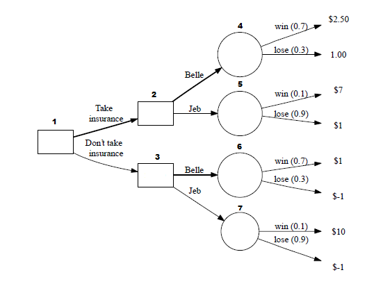
Let’s calculate some of these values. How much money could be made if we take the insurance, bet on Jeb, and then Jeb loses?:
You get paid $2 upfront for getting insurance. You bet on Jeb, so that costs you $1 upfront. You lose so you don’t have to pay them any of your earnings since you didn’t earn anything.
($2 - $1 = $1)
You will earn $1 for buying insurance, betting on Jeb, and him losing.
Let’s try another calculation. Let’s calculate how much money could be made if we don’t take the insurance, bet on Belle, and then she wins:
($2 - $1 = $1)
You will earn $1 for buying insurance, betting on Jeb, and him losing.
Let’s try another calculation. Let’s calculate how much money could be made if we don’t take the insurance, bet on Belle, and then she wins:
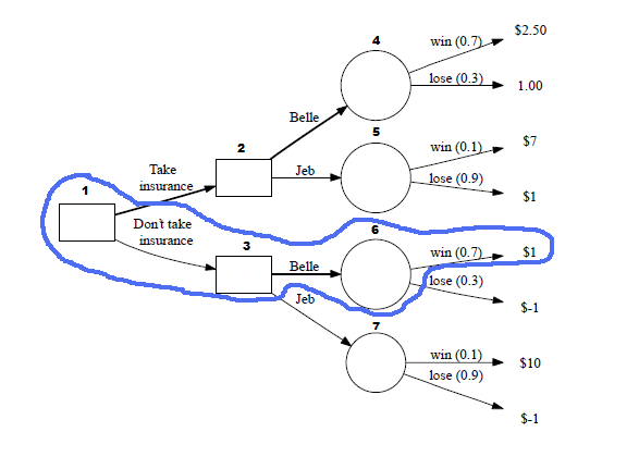
You don’t get insurance, so you don’t have to pay them anything. You bet on Belle, so that costs you $1 upfront. She wins, so you win $2.
(-$1 + $2 = $1)
You will earn $1 for not buying insurance, betting on Belle, and her winning.
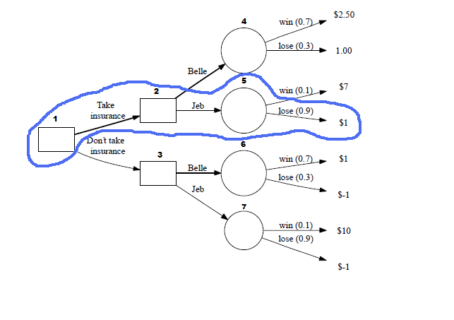
Once you’ve found all of the values for each ending branch, you can then work backward. To figure out each of the values for the circle nodes, you multiply the ending branch values by their likelihood. For example, to find out how profitable it is to bet on Belle while not getting insurance:
(-$1 + $2 = $1)
You will earn $1 for not buying insurance, betting on Belle, and her winning.
Once you’ve found all of the values for each ending branch, you can then work backward. To figure out each of the values for the circle nodes, you multiply the ending branch values by their likelihood. For example, to find out how profitable it is to bet on Belle while not getting insurance:
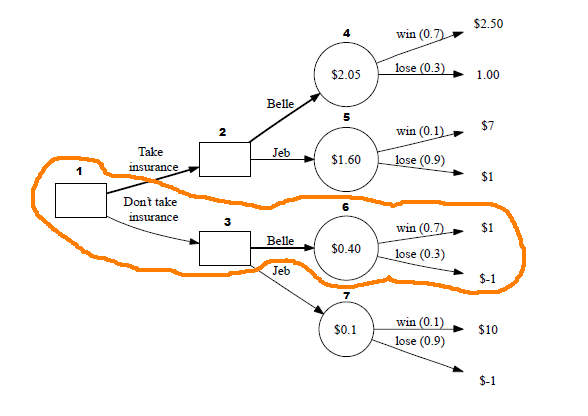
You would multiply ($1*0.7) + (-$1*0.3) = $0.40. This shows us how much we can expect to gain factoring in the fact that Belle could either win or lose.
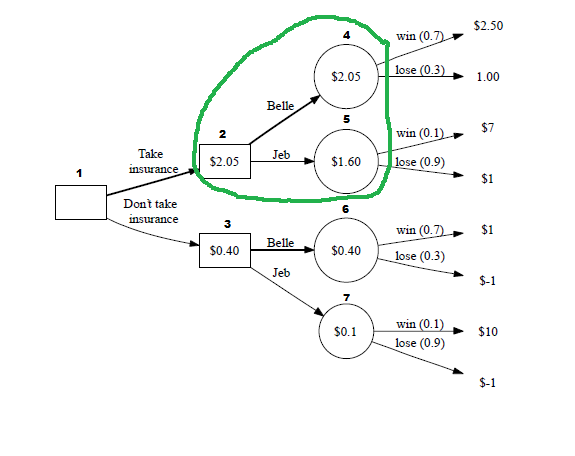
After filling in these 4 nodes, we then see which node, (4 = Belle and 5 = Jeb) has a higher expected profit, and we write that number in square node 2. Since it is belle, we write $2.50 in node 2:
After filling in these 4 nodes, we then see which node, (4 = Belle and 5 = Jeb) has a higher expected profit, and we write that number in square node 2. Since it is belle, we write $2.50 in node 2:
We do the same for node 3, but with $0.40:
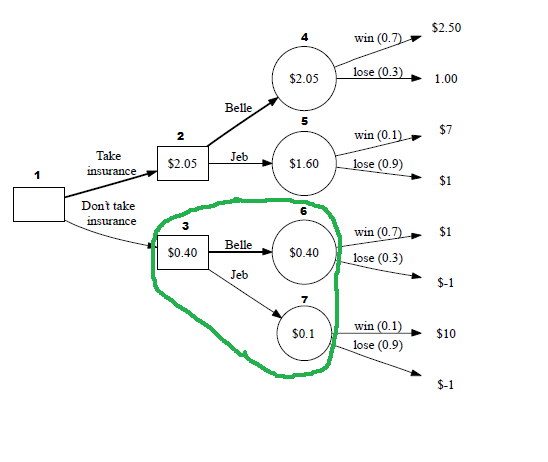
Finally, our end result is the number in node 2 or 3 that has the higher expected value. In this case, it is node 2 with $2.05:
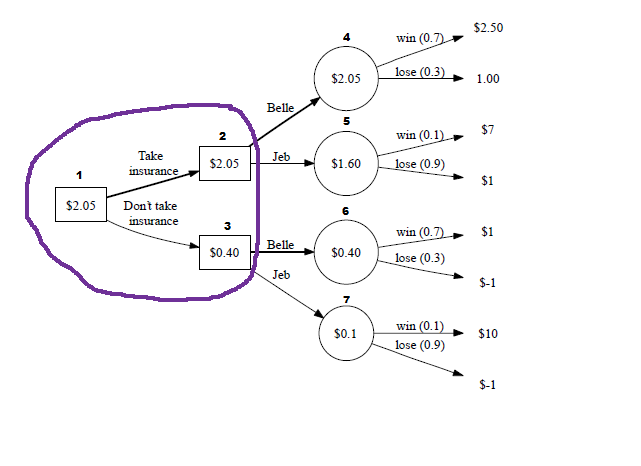
This leads us to our answer: we should take the insurance and bet on Belle (4).
